How To Create Month In Excel

Today I will show how you can create a series of automatic rolling months in Excel and then arrange your data according to the series created.

---

Download Practice Workbook

---

Creating Automatic Rolling Months in Excel

You can create a series of Automatic Rolling Months in 3 ways.

---

1. Using Fill Handle

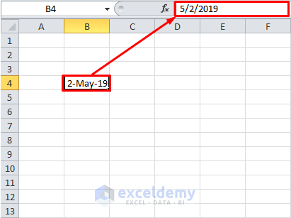
This is the easiest method. First, select a cell and enter the first date of the series you want to create. Here I select cell B4 enter 02-May-2019.

Then drag the Fill Handle upto the length of the series you want to create. Here I want to create a series of 18 cells upto cell B21.

Now from the Auto Fill Options, choose Fill Months.

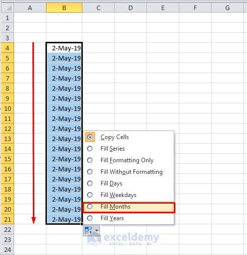
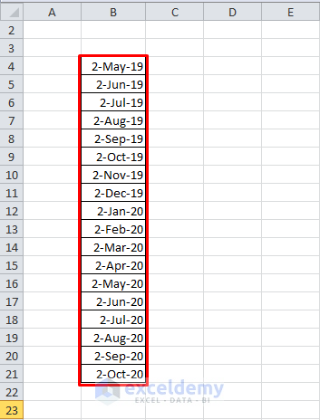
You will find a series of dates rolling by month created beautifully like this.

---

2. Using Fill Option from Excel Toolbar

You can create a series of dates of automatic rolling months by using Fill Option from Excel Toolbar.

First of all, select a cell and enter the first date of the series.

Like the previous one, I selected cell B4 and entered 2-May-19.

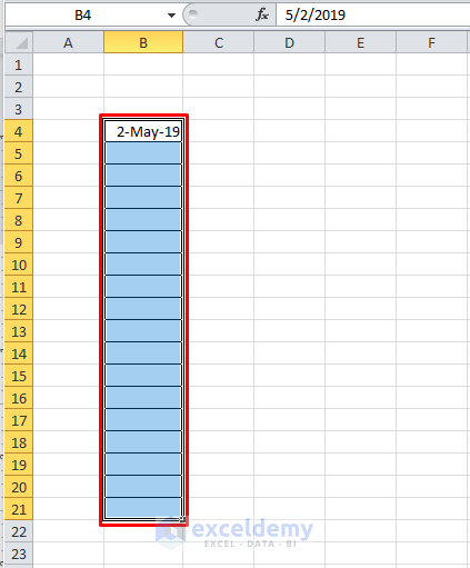
Then select all the cells where you want to insert the series. Here I select cells B4 to B21.

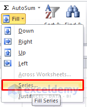
Then go to the Home>Fill option under the Editing Section of Excel Toolbar. Click the drop down menu.

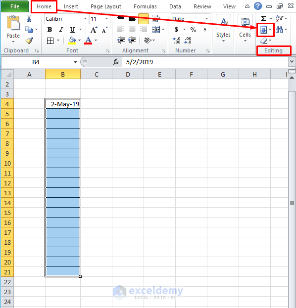
From the options available, select Series.

You will get a dialogue box called Series.

In the Series in options, check Columns.

Then in the Type options, check Date.

And then in the Date unit option, check Month.

And in the Step value box, put 1.

Then click OK.

You will find a series of dates rolling by month created beautifully like this.

---

3. Using Excel Formula

You can also use Excel formulas to create a series of dates rolling by months.

First select a cell and enter the first date.

Here I select B4 and enter the date 02-May-2019.

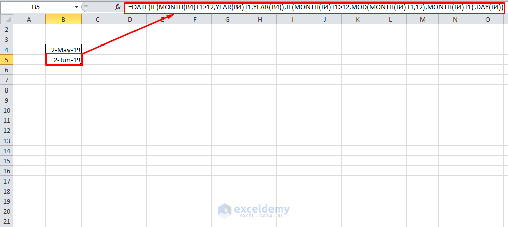
Then put this formula in the cell B5

=DATE(IF(MONTH(B4)+1>12,YEAR(B4)+1,YEAR(B4)),IF(MONTH(B4)+1>12,MOD(MONTH(B4)+1,12),MONTH(B4)+1),DAY(B4))

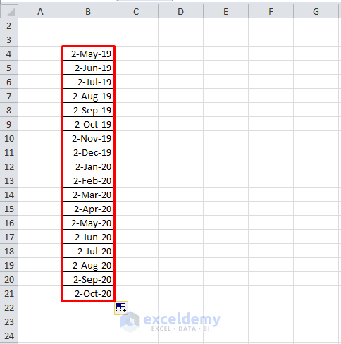
Then drag the Fill Handle up to the cell in which you fill the series. I drag them up to cell B21.

And find all the cells filled beautifully with automatic rolling months.

Note: Here B4 is the cell where I entered the first date. You can change it according to your wish and prepare the formula accordingly.

Let us explain the formula now.

• Here MONTH(B4)+1 denotes the next month of the month of B4. For example, if B4 contains month May, MONTH(B4)+1 will denote month June.
• But if the  month of cell B4 is December, that means MONTH(B4)=12,  we can not use MONTH(B4+1)=13 to go to the next month. In that case we have to come back to January with the year increased by one.
• The two IF functions within the formula do exactly the same thing.
• IF(MONTH(B4)+1>12,YEAR(B4)+1,YEAR(B4) returns the same year if MONTH(B4)+1 is less than or equal to 12, and increases the year by one if it is greater than 12.
• And IF(MONTH(B4)+1>12,MOD(MONTH(B4)+1,12),MONTH(B4)+1),DAY(B4) returns the next month if the present month is anything but December, but returns the next month as January if the present month is December.
• Finally, the year, month and the date is confined within a DATE() function to get the complete date.

---

How to Arrange Data According to the Automatic Rolling Months Created

Now come to the next stage. Let us have a look at this data set.

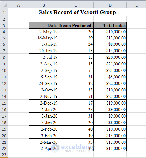
We have the Dates, Number of items produced and Total Sales in column B, C and D respectively.

Now if the CEO of the company wants to extract the record of the number of items produced and total sales on the 2nd instant of each month, how can he achieve that?

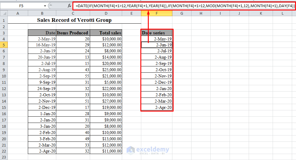
Very simple.  First create a series of the dates of the 2nd instants of every month in a new column.

I make it in column F and name it as Date Series.

The formula will be

=DATE(IF(MONTH(F4)+1>12,YEAR(F4)+1,YEAR(F4)),IF(MONTH(F4)+1>12,MOD(MONTH(F4)+1,12),MONTH(F4)+1),DAY(F4))

Then in the adjacent column G, in the cell G4, enter this formula

=INDEX(C4:C22,MATCH(F4,B4:B22,0),1)

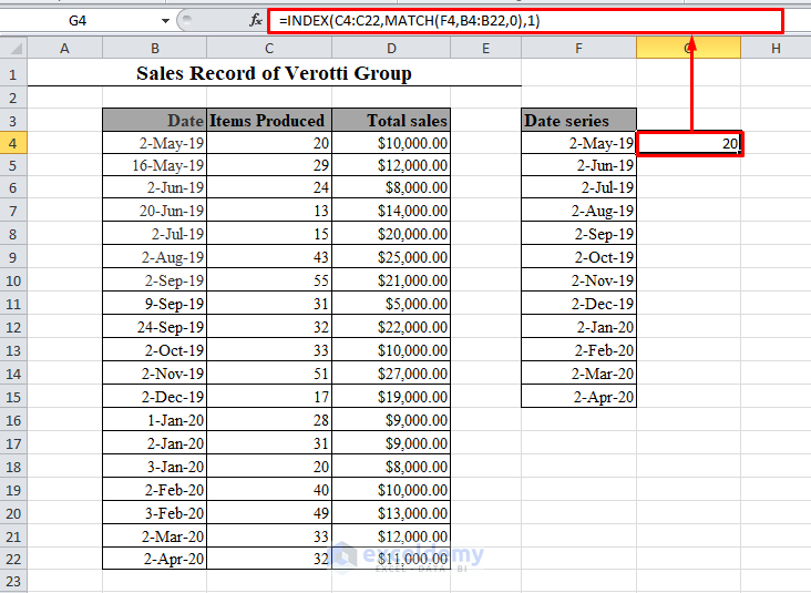
See we have extracted out the number of items produced on 2-May-19. It was 20.

Now drag the Fill Handle through the rest of the cells to extract the number of items produced on the 2nd instants of each month.

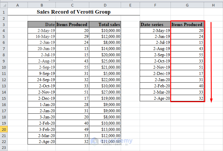
Do the same for Total Sales in column H. The formula will be

=INDEX(D4:D22,MATCH(F4,B4:B22,0),1)

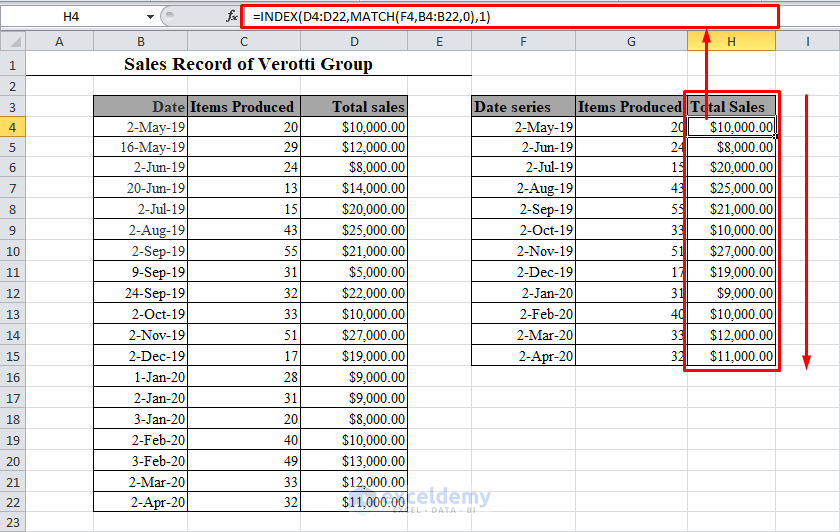
Thus we have extracted the total sales on the 2nd instants of each month.

---

Conclusion

So, using these methods, you can create a series of dates of automatic rolling months in Excel, as well as extract data from that series in Excel. Do you have any questions? Feel free to ask in the comment section.

---

Further Readings

• Excel Increment Month by 1 [6 Handy Ways]

How To Create Month In Excel

Source: https://www.exceldemy.com/automatic-rolling-months-in-excel/

Posted by: epleymisibromes.blogspot.com

Share this post